Very good feature to have in MS Excel is a dynamic drop down list when it is possible to add additional options to drop down with less efforts. So how to do it.
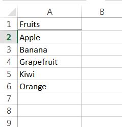
First of all lets make a source which will feed our drop down list. I decided to have some fruits in my drop down list.
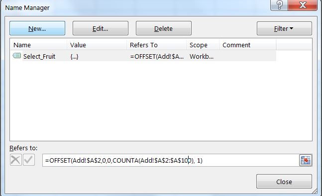
The next step would be do define that list in the name manager.

To define it we are going to use OFFSET function. In my case I have my list in a sheet called “Add” as like to call sheets where I put some additional stuff “Add” or “Additional”.
So the whole formula would be =OFFSET(Add!$A$2,0,0,COUNTA(Add!$A$2:$A$100), 1)
In this case it is possible to have up to one hundred option in the drop down list. Which is barely possible as it wouldn’t be very convenient. Function OFFSET makes that named range dynamic and I’ve named it as “Select_Fruit”.
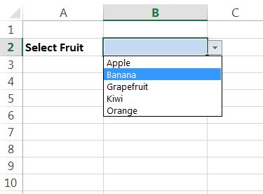
Now pick the cell where our drop down list should be. I chose cell B2, added some border and color to make it more visible.

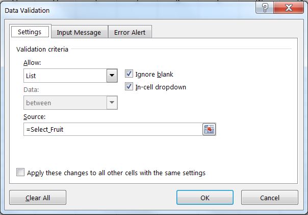
Time to add to that cell drop down list. We should go to “Data” then “Data Validation” and pick “Date Validation…”.

In Data Validation menu from “Allow” list we have to pick List.
As a Source we have to write the name we gave in the name manager which is “Select_Fruit”. Press OK and you are done.
Now you have dynamic drop down list and you can additional option by typing more name of the fruits in a sheet “Add”.
Good luck with having your own drop down list and be creative and stay smart.